vtki demo

The example demonstrates the how to use the VTK interface via the vtki library. To run this example, you will need to install vtki.

• contributed by @banesullivan

Using the inversion result from the example notebook plot_laguna_del_maule_inversion.ipynb

import os
import shutil
import tarfile
import shelve
import tarfile
import discretize
import vtki
import numpy as np

Download and load data

In the following we load the mesh and Lpout that you would get from running the laguna-del-maule inversion notebook as well as some of the raw data for the topography surface and gravity observations.

# Download Topography and Observed gravity data
url = "https://storage.googleapis.com/simpeg/Chile_GRAV_4_Miller/Chile_GRAV_4_Miller.tar.gz"
downloads = discretize.utils.download(url, overwrite=True)
basePath = downloads.split(".")[0]

# unzip the tarfile
tar = tarfile.open(downloads, "r")
tar.extractall()
tar.close()

# Download the inverted model
f = discretize.utils.download(
    "https://storage.googleapis.com/simpeg/laguna_del_maule_slicer.tar.gz"
)
tar = tarfile.open(f, "r")
tar.extractall()
tar.close()

with shelve.open('./laguna_del_maule_slicer/laguna_del_maule-result') as db:
    mesh = db['mesh']
    Lpout = db['Lpout']

# Load the mesh/data
mesh = discretize.TensorMesh.copy(mesh)
models = {'Lpout':Lpout}

Create vtki data objects

Here we start making vtki data objects of all the spatially referenced data.

# Get the ``vtki`` dataset of the inverted model
dataset = mesh.toVTK(models)

# Load topography points from text file as XYZ numpy array
topo_pts = np.loadtxt('Chile_GRAV_4_Miller/LdM_topo.topo', skiprows=1)
# Create the topography points and apply an elevation filter
topo = vtki.PolyData(topo_pts).elevation()

# Load the gravity data from text file as XYZ+attributes numpy array
grav_data = np.loadtxt('Chile_GRAV_4_Miller/LdM_grav_obs.grv', skiprows=1)
print('gravity file shape: ', grav_data.shape)
# Use the points to create PolyData
grav = vtki.PolyData(grav_data[:,0:3])
# Add the data arrays
grav.point_arrays['comp-1'] = grav_data[:,3]
grav.point_arrays['comp-2'] = grav_data[:,4]

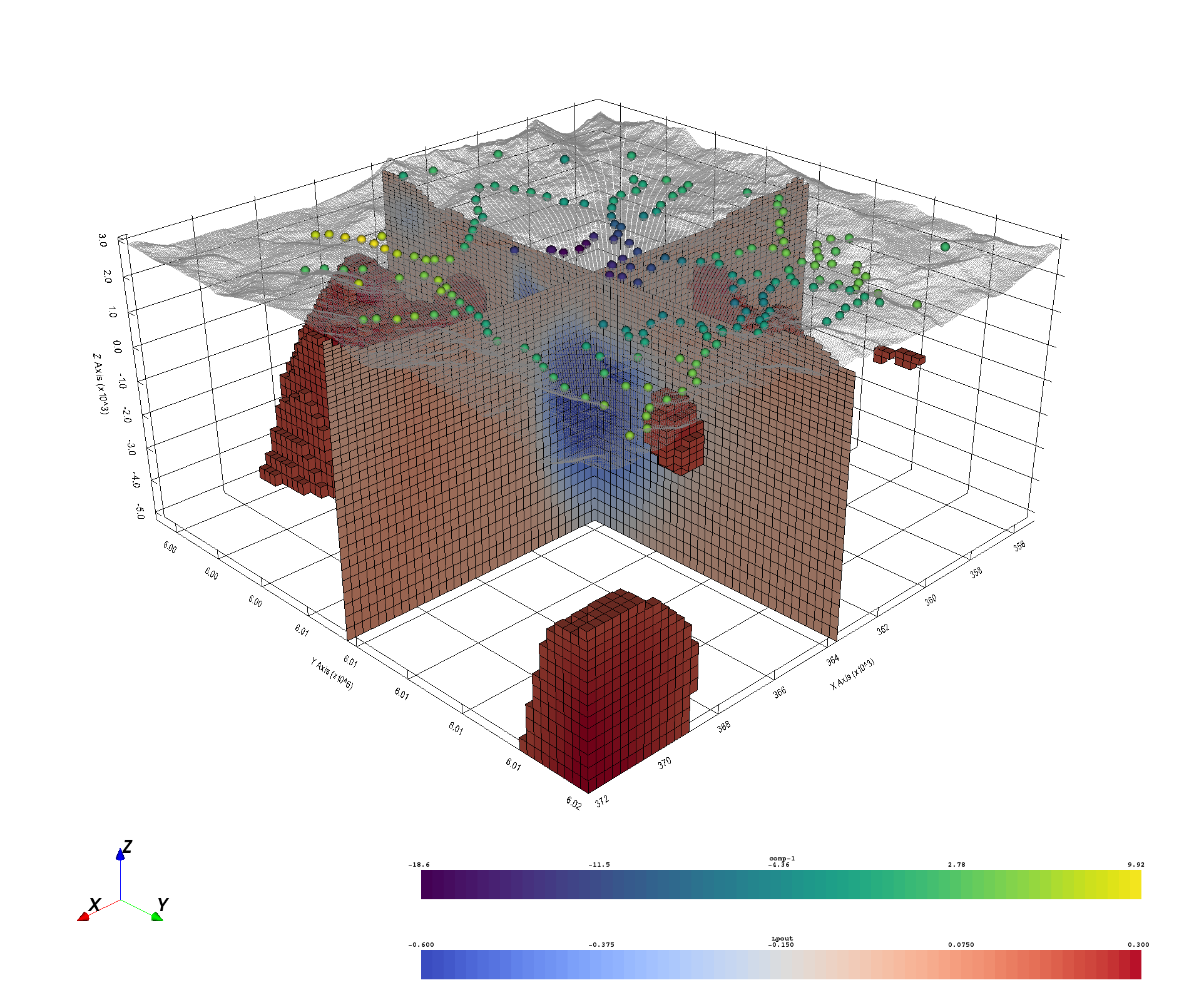
Visualize Using vtki

Here we start making visualizing all the data in 3D!

# Apply a threshold filter to remove topography
dataset_t = dataset.threshold()

# Set a documentation friendly plotting theme
vtki.set_plot_theme('document')

# Create the rendering scene
p = vtki.Plotter()
# add a grid axes
p.add_bounds_axes(grid=True, location='outer')

# Add spatially referenced data to the scene
p.add_mesh(dataset_t.slice('x'), name='x-slice', show_edges=True)
p.add_mesh(dataset_t.slice('y'), name='y-slice', show_edges=True)
p.add_mesh(dataset_t.threshold(0.2,), name='vol', show_edges=True)
p.add_mesh(topo, name='topo', color='grey',
           #cmap='gist_earth', rng=[1.7e+03, 3.104e+03],
           point_size=1, opacity=0.75,)
p.add_mesh(grav, name='gravity', cmap='viridis',
           render_points_as_spheres=True, point_size=15)

# Here is a nice camera position we manually found:
cpos = [(395020.7332989303, 6039949.0452080015, 20387.583125699253),
 (364528.3152860675, 6008839.363092581, -3776.318305935185),
 (-0.3423732500124074, -0.34364514928896667, 0.8744647328772646)]
p.camera_position = cpos

# Show the scene!
p.show(window_size=[1924, 1598], auto_close=False)

# Save a screenshot:
#p.screenshot('vtki_laguna_del_maule.png')

# Finally, close the plotter.
p.close()

Total running time of the script: ( 0 minutes 0.000 seconds)