Overview of mesh types

discretize provides a numerical grid on which to solve differential equations. Each mesh type has a similar API to make switching between different meshes relatively simple.

Within discretize, all meshes are classes that have properties like the number of cells nC, and methods, like plotGrid.

import numpy as np
import discretize
import matplotlib.pyplot as plt

General categories of meshes

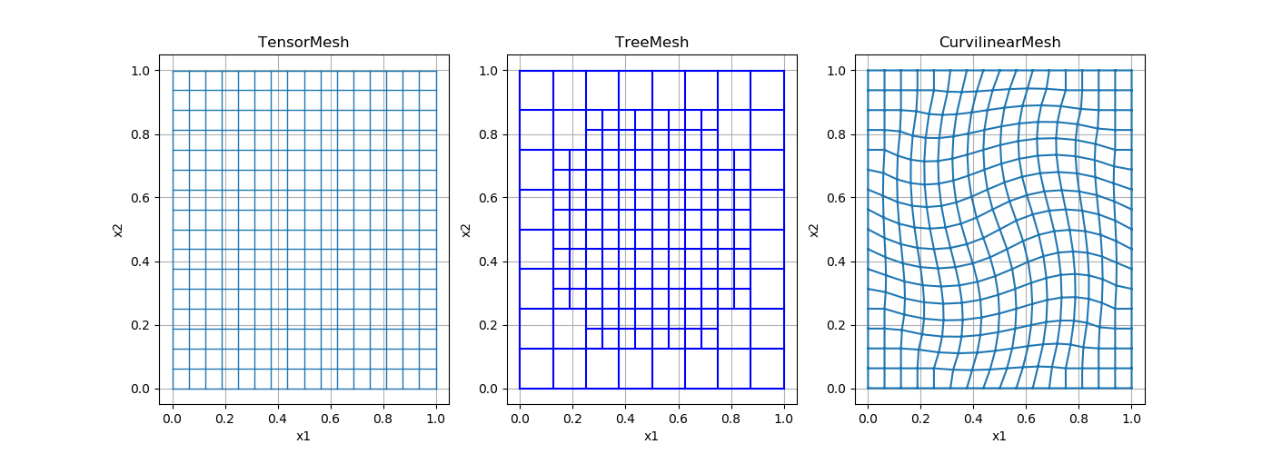
The three main types of meshes in discretize are

• TensorMesh (discretize.TensorMesh): includes cylindrical meshes (discretize.CylMesh)
• TreeMesh (discretize.TreeMesh): also referred to as QuadTree or OcTree meshes
• CurvilinearMesh (discretize.CurviMesh): also referred to as logically rectangular

ncx = 16  # number of cells in the x-direction
ncy = 16  # number of cells in the y-direction

# create a tensor mesh
tensor_mesh = discretize.TensorMesh([ncx, ncy])

# create a tree mesh and refine some of the cells
tree_mesh = discretize.TreeMesh([ncx, ncy])

def refine(cell):
    if np.sqrt(((np.r_[cell.center]-0.5)**2).sum()) < 0.4:
        return 4
    return 3

tree_mesh.refine(refine)


# create a tree mesh and refine some of the cells
curvi_mesh = discretize.CurvilinearMesh(
    discretize.utils.exampleLrmGrid([ncx, ncy], 'rotate')
)


fig, axes = plt.subplots(1, 3, figsize=(14, 5))
tensor_mesh.plotGrid(ax=axes[0])
axes[0].set_title('TensorMesh')

tree_mesh.plotGrid(ax=axes[1])
axes[1].set_title('TreeMesh')

curvi_mesh.plotGrid(ax=axes[2])
axes[2].set_title('CurvilinearMesh')

Variable Locations and Terminology

We will go over the basics of using a TensorMesh, but these skills are transferable to the other meshes available in discretize.

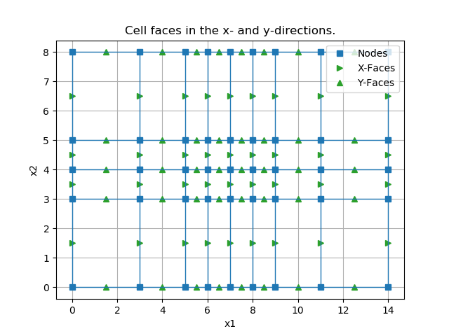
To create a TensorMesh we need to create mesh tensors, the widths of each cell of the mesh in each dimension. We will call these tensors h, and these will be define the constant widths of cells in each dimension of the TensorMesh.

hx = np.r_[3,2,1,1,1,1,2,3]
hy = np.r_[3,1,1,3]
tensor_mesh2 = discretize.TensorMesh([hx, hy])
tensor_mesh2.plotGrid(faces=True, nodes=True)
plt.title('Cell faces in the x- and y-directions.')
plt.legend(('Nodes', 'X-Faces', 'Y-Faces'))

How many of each?

When making variables that live in each of these locations, it is important to know how many of each variable type you are dealing with. discretize makes this pretty easy:

print(tensor_mesh2)

Out:

---- 2-D TensorMesh ----
   x0: 0.00
   y0: 0.00
  nCx: 8
  nCy: 4
   hx: 3.00,  2.00,  4*1.00,  2.00,  3.00,
   hy: 3.00,  2*1.00,  3.00,

count = {
    'n_cells': tensor_mesh2.nC,
    'n_cells_x_dir': tensor_mesh2.nCx,
    'n_cells_y_dir': tensor_mesh2.nCy,
    'n_cells_vector': tensor_mesh2.vnC
}

print(
    "This mesh has {n_cells} which is {n_cells_x_dir} * {n_cells_y_dir}!!".format(
        **count
    )
)

Out:

This mesh has 32 which is 8 * 4!!

print(count)

Out:

{'n_cells': 32, 'n_cells_x_dir': 8, 'n_cells_y_dir': 4, 'n_cells_vector': array([8, 4])}

discretize also counts the nodes, faces, and edges.

• Nodes: mesh.nN, mesh.nNx, mesh.nNy, mesh.nNz, mesh.vnN
• Faces: mesh.nF, mesh.nFx, mesh.nFy, mesh.nFz, mesh.vnF, mesh.vnFx, mesh.vnFy, mesh.vnFz
• Edges: mesh.nE, mesh.nEx, mesh.nEy, mesh.nEz, mesh.vnE, mesh.vnEx, mesh.vnEy, mesh.vnEz

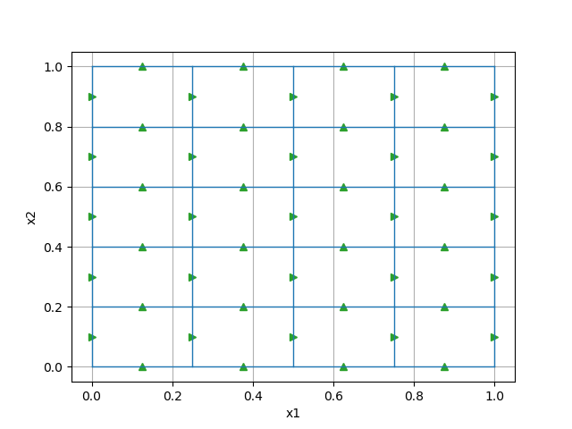
Face and edge variables have different counts depending on the dimension of the direction that you are interested in. In a 4x5 mesh, for example, there is a 5x5 grid of x-faces, and a 4x6 grid of y-faces. You can count them below! As such, the vnF(x,y,z) and vnE(x,y,z) properties give the vector grid size.

discretize.TensorMesh([4,5]).plotGrid(faces=True)

Making Tensors

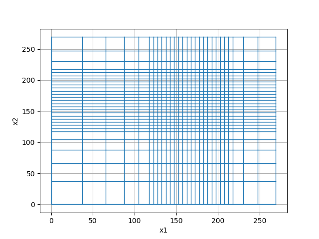
For tensor meshes, there are some additional functions that can come in handy. For example, creating mesh tensors can be a bit time consuming, these can be created speedily by just giving numbers and sizes of padding. See the example below, that follows this notation:

h = (
      (cell_size, n_pad, [, increase_factor]),
      (cell_size, n_core),
      (cell_size, n_pad, [, increase_factor])
    )

h = [(10, 5, -1.3), (5, 20), (10, 3, 1.3)]
mesh = discretize.TensorMesh([h, h])
mesh.plotGrid(showIt=True)

Total running time of the script: ( 0 minutes 0.097 seconds)