Slicer demo

The example demonstrates the plot_3d_slicer

• contributed by @prisae

Using the inversion result from the example notebook plot_laguna_del_maule_inversion.ipynb

In the notebook, you have to use %matplotlib notebook.

# %matplotlib notebook
import shelve
import discretize
import numpy as np
import tarfile
import matplotlib.pyplot as plt
from matplotlib.colors import SymLogNorm
import sys

if sys.version_info[0] < 3:
    print("This example only runs on Python 3")
    sys.exit(0)

Download and load data

In the following we load the mesh and Lpout that you would get from running the laguna-del-maule inversion notebook.

f = discretize.utils.download(
    "https://storage.googleapis.com/simpeg/laguna_del_maule_slicer.tar.gz"
)
tar = tarfile.open(f, "r")
tar.extractall()
tar.close()

with shelve.open('./laguna_del_maule_slicer/laguna_del_maule-result') as db:
    mesh = db['mesh']
    Lpout = db['Lpout']

Out:

file already exists, new file is called /Users/lindseyjh/git/simpeg/discretize/examples/laguna_del_maule_slicer.tar.gz
Downloading https://storage.googleapis.com/simpeg/laguna_del_maule_slicer.tar.gz
   saved to: /Users/lindseyjh/git/simpeg/discretize/examples/laguna_del_maule_slicer.tar.gz
Download completed!

Case 1: Using the intrinsinc functionality

1.1 Default options

mesh.plot_3d_slicer(Lpout)

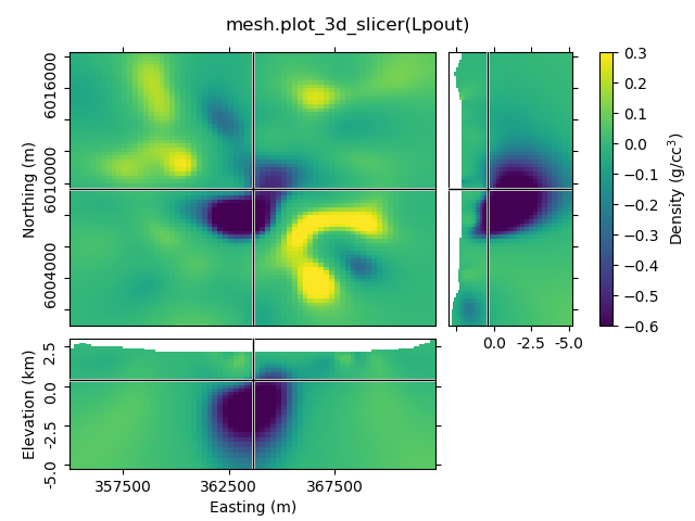
1.2 Create a function to improve plots, labeling after creation

Depending on your data the default option might look a bit odd. The look of the figure can be improved by getting its handle and adjust it.

def beautify(title, fig=None):
    """Beautify the 3D Slicer result."""

    # Get figure handle if not provided
    if fig is None:
        fig = plt.gcf()

    # Get principal figure axes
    axs = fig.get_children()

    # Set figure title
    fig.suptitle(title, y=.95, va='center')

    # Adjust the y-labels on the first subplot (XY)
    plt.setp(axs[1].yaxis.get_majorticklabels(), rotation=90)
    for label in axs[1].yaxis.get_ticklabels():
        label.set_visible(False)
    for label in axs[1].yaxis.get_ticklabels()[::3]:
        label.set_visible(True)
    axs[1].set_ylabel('Northing (m)')

    # Adjust x- and y-labels on the second subplot (XZ)
    axs[2].set_xticks([357500, 362500, 367500])
    axs[2].set_xlabel('Easting (m)')

    plt.setp(axs[2].yaxis.get_majorticklabels(), rotation=90)
    axs[2].set_yticks([2500, 0, -2500, -5000])
    axs[2].set_yticklabels(['$2.5$', '0.0', '-2.5', '-5.0'])
    axs[2].set_ylabel('Elevation (km)')

    # Adjust x-labels on the third subplot (ZY)
    axs[3].set_xticks([2500, 0, -2500, -5000])
    axs[3].set_xticklabels(['', '0.0', '-2.5', '-5.0'])

    # Adjust colorbar
    axs[4].set_ylabel('Density (g/cc$^3$)')

    # Ensure sufficient margins so nothing is clipped
    plt.subplots_adjust(bottom=0.1, top=0.9, left=0.1, right=0.9)

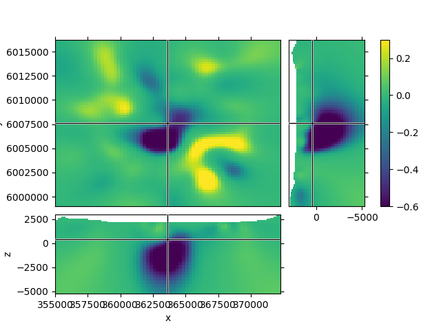
mesh.plot_3d_slicer(Lpout)
beautify('mesh.plot_3d_slicer(Lpout)')

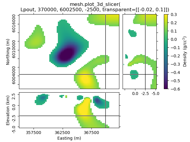
1.3 Set xslice, yslice, and zslice; transparent region

The 2nd-4th input arguments are the initial x-, y-, and z-slice location (they default to the middle of the volume). The transparency-parameter can be used to define transparent regions.

mesh.plot_3d_slicer(Lpout, 370000, 6002500, -2500, transparent=[[-0.02, 0.1]])
beautify(
    'mesh.plot_3d_slicer('
    '\nLpout, 370000, 6002500, -2500, transparent=[[-0.02, 0.1]])'
)

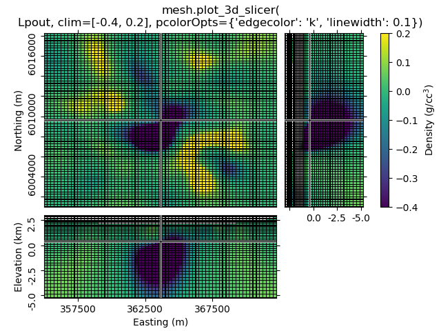
1.4 Set clim, use pcolorOpts to show grid lines

mesh.plot_3d_slicer(
    Lpout, clim=[-0.4, 0.2], pcolorOpts={'edgecolor': 'k', 'linewidth': 0.1}
)
beautify(
    "mesh.plot_3d_slicer(\nLpout, clim=[-0.4, 0.2], "
    "pcolorOpts={'edgecolor': 'k', 'linewidth': 0.1})"
)

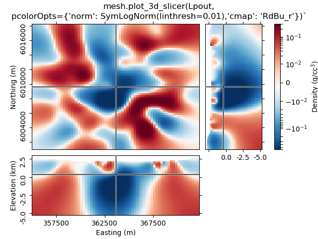
1.5 Use pcolorOpts to set SymLogNorm, and another cmap

mesh.plot_3d_slicer(
    Lpout, pcolorOpts={'norm': SymLogNorm(linthresh=0.01),'cmap': 'RdBu_r'}
)
beautify(
    "mesh.plot_3d_slicer(Lpout,"
    "\npcolorOpts={'norm': SymLogNorm(linthresh=0.01),'cmap': 'RdBu_r'})`"
)

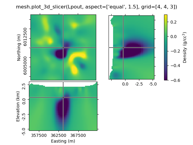
1.6 Use aspect and grid

By default, aspect='auto' and grid=[2, 2, 1]. This means that the figure is on a 3x3 grid, where the xy-slice occupies 2x2 cells of the subplot-grid, xz-slice 2x1, and the zy-silce 1x2. So the grid=[x, y, z]-parameter takes the number of cells for x, y, and z-dimension.

grid can be used to improve the probable weired subplot-arrangement if aspect is anything else than auto. However, if you zoom then it won’t help. Expect the unexpected.

mesh.plot_3d_slicer(Lpout, aspect=['equal', 1.5], grid=[4, 4, 3])
beautify("mesh.plot_3d_slicer(Lpout, aspect=['equal', 1.5], grid=[4, 4, 3])")

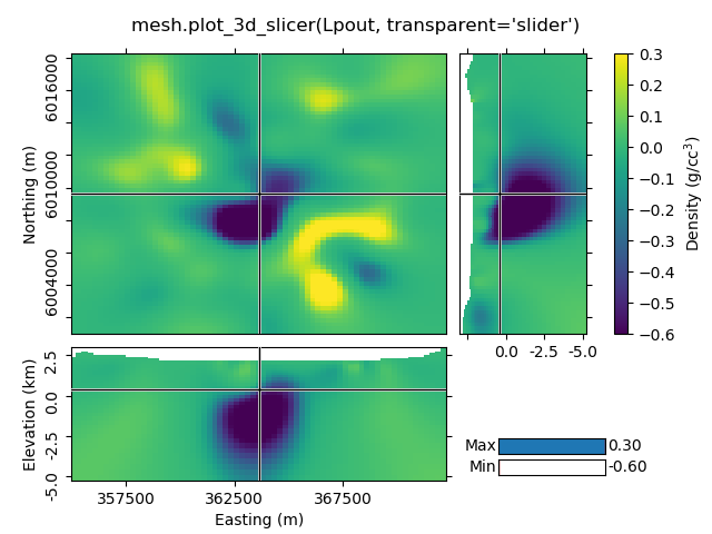
1.7 Transparency-slider

Setting the transparent-parameter to ‘slider’ will create interactive sliders to change which range of values of the data is visible.

mesh.plot_3d_slicer(Lpout, transparent='slider')
beautify("mesh.plot_3d_slicer(Lpout, transparent='slider')")

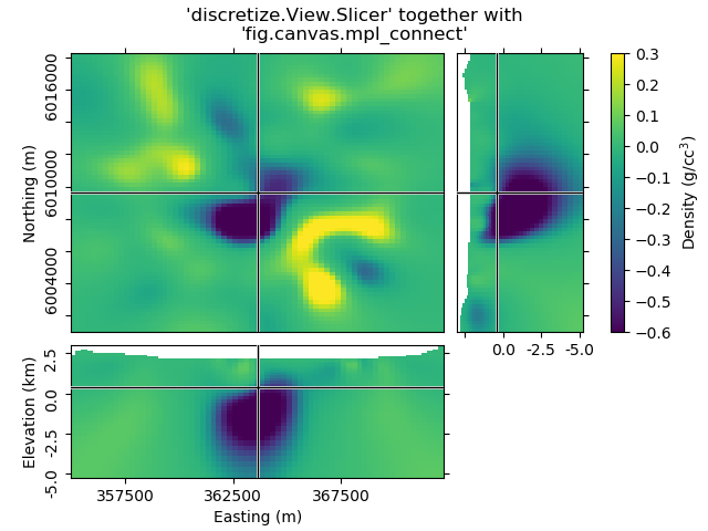
Case 2: Just using the Slicer class

This way you get the figure-handle, and can do further stuff with the figure.

# You have to initialize a figure
fig = plt.figure()

# Then you have to get the tracker from the Slicer
tracker = discretize.View.Slicer(mesh, Lpout)

# Finally you have to connect the tracker to the figure
fig.canvas.mpl_connect('scroll_event', tracker.onscroll)

# Run it through beautify
beautify(
    "'discretize.View.Slicer' together with\n'fig.canvas.mpl_connect'", fig
)

plt.show()

Total running time of the script: ( 0 minutes 1.916 seconds)